Review Deep Learning

2018-06-11 DL 0 Word Count: 791(words) Read Count: 4(minutes)

DL Basics

Linear Algebra

Scalars

Vectors

$\mathbb{R^n}$

Matrices

2-D Array

$\mathbb{R^{m\times n}}$

Tensors

Matrix Transpose

$(AB)^T=B^TA^T$

Matrix (Dot) Product

Identity Matrix

$I_nx=x$

Systems of Equations

只有一个解：可逆

Matrix Inversion

可逆必要条件：方阵，满秩

Norms

$||x||_1=\sum_i|x_i|$

$||x||_ \infty =\max\limits_i|x_i|$

Special Matrices and Vectors

正交阵：$A^{-1}=A^T$

Eigendecomposition

每一个实对称矩阵都有实，正交特征分解：

$A=Q \land Q^T$

SVD

不用是方阵

Moore-Penrose Pseudoinverse

？？？

Trace

Probability and Information Theory

Computing Marginal Probability with Sum Rule

$P(X=x)=\sum_yP(X=x|Y=y)$

$p(x)=\int p(x,y)dy$

Bernoulli Distribution

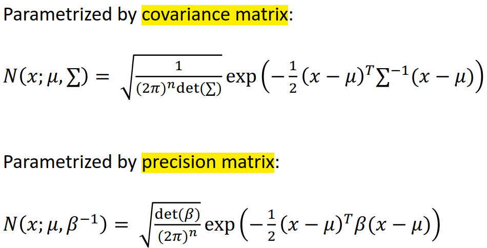
Gaussian Distribution

CNN

特点

Sparse interactions

不是全链接，稀疏链接
Parameter sharing

整张图片共享一个kernel参数矩阵
Equivariant representations

$f(g(x))=g(f(x))$

Images: If we move an object in the image, its representation will move the same amount in the output

Convolution is not equivariant to other operations such as change in scale or rotation
Ability to work with inputs of variable size

Pooling优点

Pooling helps the representation become slightly invariant to small translations of the input(we care more about whether a certain feature is present rather than exactly where it is)
Since pooling is used for downsampling, it can be used to handle inputs of varying sizes

Convolution

输出大小:

$\frac{N-K}{S}+1$

$N，原图大小(长或者宽)，K，kernel，S，步长$

Zero Padding

$\frac{K-1}{2}\ padding可以保留原来的size$

RNN

LSTM

Challenge of Long-Term Dependencies：梯度消失或爆炸

LSTM可以解决梯度消失（开忘记门），不能解决梯度爆炸

The influence never disappears unless forget gate is closed

No Gradient vanishing (If forget gate is opened.)

Instead of computing new state as a matrix product with the old state, it rather computes the difference between them. Expressivity is the same, but gradients are better behaved.

结构：

GRU结构

Exploding is controlled with gradient clipping. Vanishing is controlled with additive interactions (LSTM)

正则化和优化

Regularization is any modification made to the learning algorithm with an intention to lower the generalization error but not the training error.

经典正则化策略

Parameter Norm Penalties

L2 norm penalty can be interpreted as a MAP Bayesian
Inference with a Gaussian prior on the weights.

L1 norm penalty can be interpreted as a
MAP Bayesian Inference with a Isotropic Laplace Distribution
prior on the weights.

Dataset Augmentation
Noise Robustness

Noise added to weights

Noise Injection on Outputs. An example is label smoothing.

Early Stopping
Parameter Sharing
Parameter Tying
Multitask Learning
Bagging
Ensemble Models
Dropout

Dropout can intuitively be explained as forcing the model to learn with missing input and hidden units.

Each time we load an example into a minibatch, we randomly sample a different binary mask to apply to all of the input and hidden units in the network.

Adversarial Training

training on adversarially perturbed examples from the training set.

优化方法

Gradient Descent
- Batch Gradient Descent
Need to compute gradients over the entire training for one update
- Stochastic Gradient Descent
Minibatching

Use larger mini-batches
Learning Rate Schedule

the learning rate is decayed linearly
Momentum

The Momentum method is a method to accelerate learning using SGD

梯度：
Nesterov Momentum
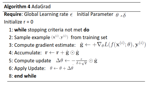
AdaGrad
RMSProp
Adam

以上方法比较

Batch Normalization

Let H be a design matrix having activations in any layer for m examples in the mini-batch

优点

Improves gradient flow through the network.
Allows higher learning rates.
Reduces the strong dependence on initialization.
Acts as a form of regularization in a funny way, and slightly reduces the need for dropout.